Radio Propagation by Tropospheric Scattering

Author: Bob Atkins - KA1GT

[This article is based on an article by KA1GT which originally appeared in the Winter 1991 edition of "Communications Quarterly]

The nature of radio wave propagation changes considerably as we move from HF through VHF/UHF and on to the microwave bands. At HF frequencies, propagation is mainly via ground wave or reflection and scattering from layers in the ionosphere. As frequency increases into the VHF and UHF region, other modes like E skip, troposcatter, meteor scatter, auroral reflection, EME transequatorial (TE) propagation, and various forms of ducting come into play. At microwave frequencies, the main propagation modes are line-of-sight, ducting, and tropospheric scatter. WlJR covered the basics of many of these propagation modes in the July and August 1986 "VHF/UHF World," columns in Ham Radio, and I refer readers to those columns for a good overview of the subject. In this article, I'd like to take a closer look at tropospheric scatter the most reliable propagation mode for working VHF/UHF/microwave DX.

Propagation modes

Line-of-sight operation will, in general, give the strongest signals for a given path length, but line-of-sight paths are limited in both number and length. Ducting, the trapping of signals in a waveguide-like duct formed by atmospheric layers of different refractive index, can propagate VHF/UHF/microwave signals with very little loss over long distances. Unfortunately, ducting is rare and relatively unpredictable, and it's difficult to calculate the magnitude, length, and frequency characteristics of a duct in advance. Propagation by E skip, auroral, and trans-equatorial modes is also unpredictable and limited in frequency and duration. Communication via meteor scatter is possible on a fairly reliable basis on the lower VHF bands, but communication time is limited to very brief intervals. EME provides the ultimate in DX, but requires special antenna systems (high gain and the ability to elevate and track the moon) and high power levels. Communication is only possible when the moon is visible to both stations. Of all the possible propagation modes, only tropospheric scatter (troposcatter) provides a reliable and predictable mode of operation for working DX on the VHF/UHF/microwave bands on a day-in, day-out basis using moderate equipment. In fact, troposcatter circuits are often used commercially when over-the-horizon communication is desired and the use of repeaters isn't possible.

A nice feature of troposcatter propagation is that it's possible to make reasonably accurate estimates of path loss. Such estimates can be instructive from a number of viewpoints.

Because the calculation is based on parameters like antenna height, local topography, and station separation it can, for example, predict what effect increased antenna height will have on signal strength. In combination with receiver and transmitter parameters, troposcatter propagation can station indicate would what be needed kind of for a VHF liaison talk-back on a DX microwave record attempt, and what the likelihood is of working a given microwave DX path.

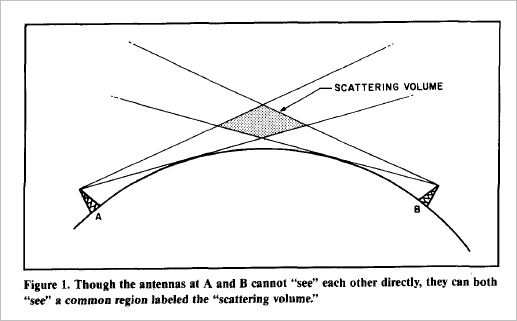
The basic mechanism of tropospheric scatter is shown in Figure 1. The antennas of the two stations at the ends of the path cannot "see" each other, but they can each "see" a common volume of the atmosphere, labeled in the figure as the "scattering volume." Signals from one station are scattered by atmospheric inhomogeneities in this region, and some of the scattering is in the direction of the second station. The region of the atmosphere involved is called the troposphere and it extends from the ground up to a height of about 15 km. It's the region in which all weather phenomena occurs, air- planes fly, and is the region in which the "air" is found. Although this region looks clear and uniform to the eye, it really contains a lot of turbulence and stratification. Anyone who has had a bumpy ride in an aircraft has felt this first hand, just as anyone who has seen a star twinkle has directly observed the optical effects of atmospheric turbulence.

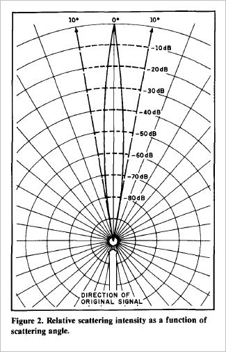
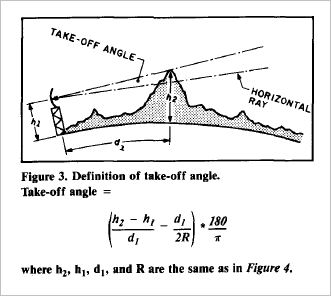
One characteristic of tropospheric scattering is that it occurs mainly in the original direction of the signal, as shown in Figure 2. As the scattering angle increases, the magnitude of the scattering falls off very rapidly (around 10 dB per degree), so the process is only useful where the scattering angle is limited to a few degrees. Two major factors are involved in determining the scattering angle between two stations. The first is the distance between the stations and the second is the "take-off angle" at the two stations. Take-off angle is defined as shown in Figure 3; that is, it's the angle between a horizontal ray from the antenna and a ray from the antenna to the radio horizon. Take-off angle has a strong influence on path loss. For a given path, a 1-degree increase in take-off angle will result in a decrease of around 10 dB (depending on the scattering model) in the received signal strength. If the take-off angles are large, then not only will the scattering angle be large, but the scattering volume will extend to high altitude, where the atmosphere is thinner and the scattering is therefore diminished.

Models for calculating path loss on troposcatter links

There have been many models developed to calculate the path loss on a troposcatter link, including those of ITT{1] NBS[2] CCIR[3] Collins[4] Yeh[5] and Rider[6] A review of these models (except for ITT) was made by Larsen[7] who found that the Collins model performed best, followed by Yeh, CCIR, and NBS, though all were capable of yielding good results. On paths ranging from 275 to 994 km at frequencies from 77 MHz to 3.7 GHz, path losses were often predicted to within a few dB. The ITT model has been shown to be very accurate on many paths? Rider's model was found to be inferior to the others. The NBS model is very complex and really requires a computer program to be practical. The CCIR method is a slightly simplified version of the NBS model, and the Collins and ITT models rely on the use of graphs which cover only a limited parameter range. This leaves Yeh's model as the best alternative for a simple computational method to determine tropospheric scatter path loss.

Yeh breaks down path loss into four basic components:

• Free space path loss
• Scattering loss
• A loss factor dependent on the refractive index of the air
• Aperture-to-medium coupling loss, which is a function of the scattering angle and the antenna beam widths used.

Taking these in turn:

Free space path loss

The free space path loss (in dB) between isotropic antennas can be calculated from first principles. Without going into details of the derivation, it can be shown to be given by the expression:

10Log₁₀(4πd/λ)²

Where d is the distance and λ is the wavelength (in the same units).

When this is rearranged and stated in customary units, it can be expressed as the well known relationship:

L_fs = 32.5 + 20log₁₀(d) + 20log₁₀(f)

Where d is the (great circle) distance in km and f is the frequency in MHz.

Scattering loss

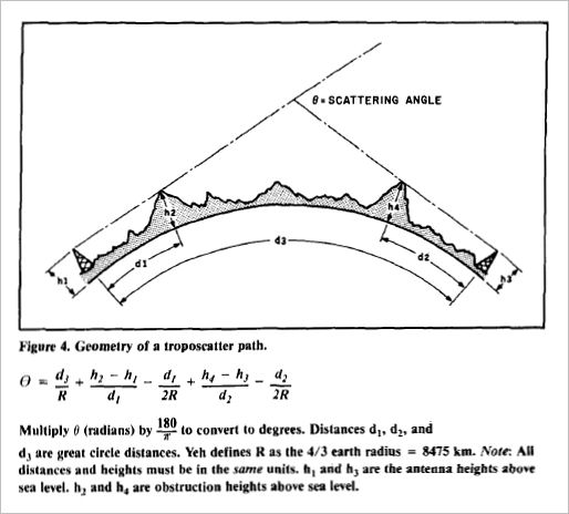
Yeh determined the scattering loss empirically based on two sets of experimental observations. The first was that scattering loss was proportional both to frequency and to the scattering angle (10 dB per degree). The second was that the scatter loss at a 1- degree scattering angle (about a 90-mile path) was 57 dB at 400 MHz. These observations may be combined to yield the relationship:

L_s = 57 + 10(θ-1) + 10log(f/400)

Where θ is the scattering angle as defined in Figure 4 and f is the frequency in MHz.

This can be simplified to:

L_s = 21 + 10(θ) + 10log(f)

The determination of θ depends on knowing the local topography around the stations at each end of the troposcatter link. It's important to determine the "take-off angle" for each station. To do so, you must know the height of the antenna and the height and location of the geographic feature which determines the local radio horizon in the direction of the distant station. Two useful websites to assist with this are:

• Geocontext Profiler
• HeyWhatsThat

Variation in the value of the radio index of refraction

The third factor is dependent on the radio refractive index of the air. This rests on a number of variables, the most important of which are air temperature and humidity. The surface refractivity, N_s is the refractive index expressed in millionths above unity. For example, if the refractive index is its nominal value of 1.000310, the value of N = 310. The value and range of variability of N_s is a function of geographical location and season. It's highest in the summer in tropical coastal regions, and lowest in the winter in the mountains.

Because N_s is dependent on atmospheric pressure, it follows that it's also a function of altitude. To avoid confusion when reporting surface refractivity values from different sites at different altitudes, it's common to give values of surface refractivity corrected to sea level - often designated as N₀. For example, in Denver, at an altitude of approximately 1.6 km above sea level, a typical value of N₀ might be given as 300. The actual surface refractivity will be lower and can be approximated by the formula:

N_s = N₀e^-0.1057h

Where h is the elevation above sea level in km.

For Denver, with h=1.6 and N₀ = 300, the surface refractivity, N_s would be 253. Though Yeh doesn't discuss how to define N_s (or calculate it from N₀) for situations

in which the surface refractivities at two sites are different, it seems reasonable to take the average of two values.

Values of N₀ in the United States can range from a low of around 260 in the Rocky Mountain region in the winter to over 380 along the coast of the Gulf of Mexico in the summer. Typica1 values for the Midwest and eastern regions of the U.S. are around 310 in the winter and 350 in the summer. A method of estimating N, from barometric pressure, temperature, and humidity data is given in References 8 and 9.

The importance of the radio refractive index lies in the fact that a higher value of N_s causes radio waves to bend back towards the earth to a greater extent. More accurately, it's the change in refractive index with height which results in this effect which can be likened to the bending of light rays passing through a graded index lens. Thus radio waves don't travel in a straight line when passing through the atmosphere, but tend to bend back slightly towards the earth. An alternative way of looking at the same phenomenon is to regard the radio waves as traveling in straight lines above an earth whose radius is larger than the true radius. This gives rise to the well-known 4/3 earth radius approximation which predicts that, under average conditions, the radio horizon is at a distance 4/3 greater than the optical horizon (or more accurately, the geometric horizon, because light rays are also bent slightly).

The increase in path loss as a function of N_s is approximated by Yeh as:

L_n = 0.2(310-N_s) (dB)

Aperture-to-medium coupling loss

The last loss factor is the aperture-to- medium coupling loss. It has been observed experimentally that, on long haul troposcatter paths, signal strength doesn't increase as much as would be predicted when antenna gains are increased. The effect is only observed for very high gain antennas, when the antenna beam width is decreased to a value close to that of the scattering angle. The mechanism of this loss is complex and not well understood. It's derived from the way in which the antennas couple with the scattering process and may be associated with phase incoherence resulting from scattering by multiple random atmospheric inhomogeneities. Yeh based his estimate of aperture-to-medium coupling loss on the results of a number of experimental studies, rather than a theoretical model. In his original paper, a graphical determination is presented which may be approximated by the relationship:

L_amc = 2.5 + 1.8(θ/α) - 0.063(θ/α)²

Where α = √(bw1*bw2)
bw1 = 3dB beamwidth of antenna 1 (in degrees)
bw2 = 3dB beamwidth of antenna 2 (in degrees)
θ = the scattering angle (in degrees

A couple of points are worth noting here. Yeh suggests that there may be some error when aperture-to-medium loss is extrapolated outside the region of experimental data, which ranges from values of θ/α of about 0.5 to 4. Extrapolating to very small values (as would often be the case using Amateur antennas of modest gain) gives a minimum value of 2.5 dB, whereas other studies show much smaller coupling loss when θ/α is small. There are a number of other empirical relationships for determining the magnitude of this loss. The value used in the CCIR method[3] is given by:

L_CCIR = 0.07e^{(0.055(G1+G2))}

Where GI and G2 are the gains (in dB) of the two antennas.

As you can see, this relationship doesn't involve the scattering angle at all. Thus, it's evident that determination of aperture-to-medium coupling loss isn't an exact science! Luckily it's of small importance, typically only a few dB, with the types of antennas Amateurs are likely to be using. For consistency with the rest of Yeh's method, his estimation of coupling loss should probably be used here.

Adding all four of the preceding loss factors together, you come up with an expression for the total loss of a troposcatter path:

L = L_fs + L_s + L_amc + L_n

or L=32.5 + 20log₁₀(d) + 20log₁₀(f) + 21 + 10(θ) + 10log₁₀(f) + 0.2(310 - N_s) + 2.5 + 1.8(θ/α) - 0.063(θ/α)²

Which reduces to:

L = 56 + 20log₁₀(d) + 30log₁₀(f) + 0.2(310 - N_s) + 10(θ) + 1.8(θ/α) - 0.063(θ/α)²

When the mean yearly value of N_s is used, the loss predicted by this expression is the all-year median (or most probable) path loss. A discussion of the statistical probability of the signal differing from this level would fill many more pages, so I won't go into that now. For a very rough rule of thumb for overland paths of 100 to 300 km in a climatic region similar to that of the continental United States, path loss will be 10 dB higher or lower than the median about 10 percent of the time and 20 dB higher or lower than the median about 1 percent of the time. Fluctuations in path loss tend to decrease as path length increases over 300 km or drops below 100 km. On average, signals will be stronger in the summer than in the winter. They will also be stronger in the early morning and late evening, when the air is turbulent due to heating and cooling, than in mid-afternoon, when the air is well mixed and stable.

Now that you have a way to calculate troposcatter loss, it's obviously of interest to ask how accurate the estimate will be. Larson[7] looked at sixteen paths ranging from 275 to 994 km at frequencies from 77 MHz to 3.67 GHz, with measured path losses ranging from 163 to 257 dB. He found that Yeh's method gave a mean error (independent of sign) of 5.9 dB. When the sign of the error was taken into account, the mean error (sum of errors/number of examples) was -3.0 dB; that is, there was a slight tendency to underestimate the path loss. The mean error of the other methods of estimating path loss referred to earlier were within a few dB of those of Yeh. This might not be surprising at first, but the methods have significant differences. For example, the Collins method has no term dependent on N,, which has a significant effect on the loss predicted by Yeh. On the other hand, both the NBS and CCIR methods contain a climate correction factor not used in any of the others! Using Yeh's method, Gannaway[10] estimates the troposcatter loss of a particular 110 km path at 10.368 GHz to be 232 dB. Averaging careful measurements over a period of months, he found an experimental path loss of 235 dB, a difference of only 3 dB.

Although Yeh doesn't discuss frequency limits in his paper, the method, as described here, is probably restricted to a range from about 50 MHz to 10 GHz. Below 50 MHz the dominant mode of DX propagation may not be troposcatter, because ionospheric reflection starts to come into play. Above 10 GHz, absorption of RF energy by oxygen and water vapor can make a significant contribution to path loss. If these losses are added to the calculated troposcatter loss, then total path loss predictions can be made at frequencies above 10 GHz. It may be noted that even below 10 GHz, atmospheric attenuation will be a small factor on long paths. For example, over 500 km, an additional loss of about 5 dB over the troposcatter loss can be expected at 10 GHz[11]

Assuming the accuracy of troposcatter prediction is quite good, it's interesting to calculate the potential communication range between two reasonably equipped stations (see Reference 12). As an example, take two stations with a capability of 100 watts output on 432 MHz, each using a single 18 dBi gain Yagi with a receiver noise figure of 1 dB and having 1 dB line loss on both transmit and receive. If both stations have an unobstructed view of the horizon (take-off angle of zero degrees), they should be able to communicate on CW over a range of 650 km. This is considerably greater than most station operators would guess, and suggests the unrealized potential of many stations.

One question which often comes up in discussions about troposcatter paths is should the antennas be elevated above the horizon in order to better illuminate the scattering volume? The answer is almost always no; the antennas should point at the horizon. Many studies have shown that when using very high gain, narrow beam width (< 1 degree) antennas, elevation even by a fraction of a degree results in signal loss. This is because elevation of the antennas increases the scattering angle. A 1 degree elevation at each end results in a 2 degree increase in scattering angle and a consequent increase of 20 dB in troposcatter path loss. The effect is significant when the antenna's beam width is of the same order as the angle of elevation. In this case, the gain in the direction of the horizon will drop drastically and so there will be little contribution to troposcatter from low altitude, low angle scattering. On the other hand, if antennas with a relatively large beam width (low gain) are elevated slightly, their gain in the direction of the horizon will drop only slightly. In this case, they will still illuminate the same low angle scattering volume with only slightly less signal than they did when they were pointed directly at the horizon, thus signals will not decrease much. However, after saying all this, there are infrequent occasions on which elevation of the antennas does lead to an increase in signal strength. This may be due to a rare circumstance when elevation of the antennas results in illumination of a high altitude, very intense scattering region of the atmosphere, such as a thunderstorm cell. In fact it has been observed that during rainstorms, microwave signals can be received by "rain scatter" with the antenna at one end of a troposcatter link pointing vertically upwards! The moral here is that when no signals at the can horizon be detected (assuming with antennas beam headings point and frequencies are known to be correct) it can't hurt to try elevating the antennas by a few degrees but don't expect it to do much good very often.

As I mentioned earlier, calculation of troposcatter loss can be used to estimate the effects of an increase in antenna height, assuming that the antenna is clear of all local obstructions (trees, buildings, etc.). For example, consider two stations 200 km apart, each with antennas on 15 meter (ca. 50 feet) towers and separated by a level plain (sounds like Kansas!). On 1296 MHz, the troposcatter path loss between these stations would be about 206.5 dB. If one station doubled the height of its tower to 30 meters, the path loss would fall to 206 dB. This is only a difference of 0.5 dB (this difference is independent of frequency), and would probably be negated by the extra feed line loss required to reach the antenna. This shows that if your antenna is in the clear, and you have a very low level horizon, there's no real advantage to be gained by increasing antenna height. This is a situation where the more cost effective solution to better signals is to increase the antenna gain.

However, let's look at a different situation where one of the stations I've described has a 30-meter (100 foot) high hill at a distance of 1 km, instead of an unobstructed horizon. If this station uses the same 15-meter high antenna, the path loss will be 216.9 dB. If the antenna is raised to 30 meters, this loss drops 208.1 dB. In this situation the increase in to signal is 8.8dB, a considerable improvement. Because this increase in signal would be realized on all the microwave (and VHF/UHF) bands, the cost-effective solution to increased signal strength in this case would be to increase the antenna height, as eight times as many antennas on each band would be required to equal the effect of a 15-meter increase in antenna height.

Another use for this type of calculation is in estimating the equipment needed to work a given path. For example, take the path between Cadillac Mountain in Maine (466 meters asl, the highest point on the Eastern seaboard) and the tip of Cape Cod in Massachusetts a distance of about 300 km. Yeh's method of troposcatter prediction indicates a path loss at 10.368 MHz of around 244 dB for this path (the other methods mentioned earlier are several dB more optimistic). Using the standard relationships between path loss and equipment parameters (see 12), it can be calculated that on 10 GHz, this path should be just workable (+1.5 dB S/N) under flat conditions using CW with a 100 mW transmitter, a 3-dB noise figure receiver, and a 3-foot dish. This setup is typical of the narrow-band equipment used by many amateurs on this band. Calculations indicate that a 144-MHz SSB talk-back link (+ 14 dB S/N) can be established for this path with 10-watt transmitters and 10-dBi gain antennas (4-element Yagis).

Program

A Windows program to calculate path loss and overall link budget for both line of sight and troposcatter paths can be downloaded from this website. See The KA1GT troposcatter program page. The file is an executable, written in Visual Basic 6. It's stand alone, meaning it makes no changes to you system, installs no DLLs and makes no registry changes.

Conclusion

In this article, I have tried not only to present a method for estimating troposcatter loss, but also to provide some physical understanding of the processes involved. The procedures outlined here, can be used as a basis for the selection of an optimum VHF/UHF/microwave site, or can give a quantitative estimate of the benefits to be gained by increasing antenna height, lowering noise figure, lowering feed line losses etc. An analysis of troposcatter loss combined with equipment path loss capabilities may reveal the unrealized potential of many stations.

Notes

Readers who want to learn more, might like to consult the references listed at the end of this article. Reference 2 probably gives the most extensive treatment of tropospheric path loss available, though much of the text is quite mathematical.

Some of the first seven references may be hard to find, even in college libraries. I can recommend the book listed in Reference 8, which includes brief reviews of some of the other references and much more very useful information. Reference 10 is an excellent treatment of Yeh's method of calculating troposcatter loss and includes a number of graphs and examples. It's recommended reading, if you can obtain a copy.

REFERENCES

I. H. Smith, ITT Federal Laboratory Technical Memorandum, June I963, pages 63-175. and R.E. Grey, ITT Federal Laboratory Technical Memorandum, October 24, 1961.

2. P.L. Rice, A.C. Longley, K.A. Norton, and A.P Barsis, NBS Technical Note 101, May I965 (revised January 1967).

3. CCIR Documents of the XIth Plenary Assembly. Oslo. l966, pages 143-167.

4. Instruction Manual for Tropospheric Scatter - Principles and Applications, USAEPG-SIG 960-67, U.S. Army Electronic Proving Ground, Fort Huachuca, Arizona, March 1960.

5. L.P. Yeh, "Simple Methods for Designing Troposcatter Circuits." IRE Transactions on Communications Systems, September 1960, pages 193-198.

6. C.C. Rider, Marconi Review, 3rd quarter 1962, pages 203-210.

7. R.A. Larsen, IEE London Tropospheric Wave Propagation Conference, 1968.

8. P.F. Panter, Communications Systems Design, McGraw-Hill.

9. Dennis Haarsager, N7DH, The ARRL UHF/Microwave Experimenter's Handbook, pages 3-37.

10. Julian Gannaway, G3YGF. "Tropospheric Scatter Propagation." Radio Communications, August 1981. Also reprinted in QST; November 1983, pages 43-48.

11. Roger Freeman, Telecommunications Transmission Handbook, John Wiley & Sons.

12. Bob Atkins, KAIGT, "Estimating Microwave System Performance," QST December 1980, page 74.